![]()

![]()
![]()
Phonon Calculations via VASP
Contents
- Prerequisites
- Overview
- 1. Cell & atom relaxation
- 2. Enforcing symmetries
- 3. Density functional perturbation theory (DFPT) calculation
- 4. Extracting mode symmetries with Phonopy
- 5. Phonon dipsersion
- 6. Phonon density of states
- 7. Free energy via Phonopy
Prerequisites
Before starting, you will want the following software:
- VASP 5.3 or greater (requires a license)
- Phonopy (see this link for download instructions)
- Access to materialsproject.com
- VESTA (not entirely necessary, but useful for mode visualizations)
Overview
 The Phonopy Python
package provides a simple interface for extracting vibrational and
thermal properties of materials from VASP output. This tutorial shows
how to use VASP and Phonopy for phonon density of states, dispersion,
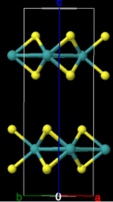
and free energy calculations. We will use bulknn MoS\(_2\) as an
example. In general, phonon calculations with VASP involve the
following steps:
The Phonopy Python
package provides a simple interface for extracting vibrational and
thermal properties of materials from VASP output. This tutorial shows
how to use VASP and Phonopy for phonon density of states, dispersion,
and free energy calculations. We will use bulknn MoS\(_2\) as an
example. In general, phonon calculations with VASP involve the
following steps:
- Relaxation of the atomic positions and/or cell
- Checking atomic positions/lattice constants to ensure cell symmetries have not been broken
- Density functional perturbation theory (DFPT) calculation of phonon modes
- Extracting modes with Phonopy
- Computing phonon density of states, dispersion, etc.
It is useful to set up different directories corresponding to steps 1 and 3.
$ ls
1-relax/  2-dfpt
The initial structures for MoS\(_2\) come from the Materials Project (mp-2815).
1. Cell & atom relaxation
Files for this section: github link
In order to get accurate phonon modes, it is necessary to first relax
the atomic positions and/or lattice constants. VASP provides several
different methods for relaxation, provided by specifying the ISIF
tag (see here for
details).
Generally, there are two different cases:
- The desired symmetry of the cell is known, but the atomic positions
and/or lattice constants are not known. In this case, you want to
enforce symmetry of the starting structure in the POSCAR file. You
should use:
IBRION = 2, ISYM = 2. The choice ofISIFalso needs to be specified. To relax atom positions only (lattice constants fixed), chooseISIF = 2. For relaxation of the lattice constants, choose eitherISIF = 3(cell volume can vary) orISIF = 4(cell volume remains fixed). - The symmetry of the initial structure is not known to be
correct. In this case, use
IBRION = 2, ISYM = 0(i.e., turn off symmetry). Usually you wantISIF = 3for this case.
After this calculation, you will want to look at the CONTCAR file
that is output. Depending on the choice of parameters in the INCAR
file, you may notice that the symmetry of the cell has changed. For
example, see the result of the second option
above
here. This
file will need to be modified further (see part 2 below) before
use in DFPT calculations.
2. Enforcing symmetries
Files for this section: github link
After performing the relaxation, it is possible that the resulting
atomic positions and lattice constants in CONTCAR will not be
symmetrized. For example, if using IBRION = 2, ISYM = 0, ISIF = 3,
you will almost certainly not have the exact same lattice constants as
you started with.
For phonon (DFPT) calculations, the lack of symmetry can eventually
lead to issues in understanding the phonon modes. For example, the
structure in CONTCAR could be very close to a hexagonal or
tetragonal unit cell, but there could be just enough difference in
the lattice constants for the cell to be classified as triclinic. This
will result in problems later on (e.g., in the assignment of
irreducible representations of the normal modes).
To ‘fix’ this problem, you may want to edit the CONTCAR file and
enforce the symmetry you desire. For example, you could see values
like -0.00001248932473 in the x,y, or z components of the lattice
constants. This should most likely be 0, so you can modify and round
to 0.00000000000000. After doing this for the lattice constants and
atomic positions, it isn’t a terrible idea to run another relaxation,
but this time with fixed lattice constants (ISIF =2) and possibly
enforcing symmetry this time (ISYM = 2). This will leave you with a
structure that has the symmetry properties that you most likely want
for phonon calculations.
3. Density functional perturbation theory (DFPT) calculation
Files for this section: github link
After relaxing the cell, you can use the final CONTCAR as input to a
phonon calculation (i.e., mv 1-relax/CONTCAR 2-dfpt/POSCAR). Phonon
modes can be computed via two different ways: density functional
perturbation theory (DFPT) and finite displacements. DFPT requires
only one simulation to get the dynamical matrix and compute all modes,
while the finite displacements method involves one or more
simulations, each displacing a single atom to compute the forces. DFPT
offers an all-in-one approach, but it also takes longer to run because
all displacements are done in a single simulation. If using a large
cell with limited wall time on a cluster, it is possible that the job
will not finish.
To perform a DFPT calculation with VASP, choose IBRION = 7 or
IBRION = 8 in the INCAR file (an example of an INCAR for DFPT is
shown below). IBRION = 8 applies symmetry operations to reduce the
number of displacements needed, while IBRION = 7 does not. The
IBRION=7 option will perform \(3N_\mathrm{atoms}\) displacements,
whereas IBRION=8 option will greatly reduce the number of
displacements based on the crystal symmetry. However, IBRION=8 does
not allow for the use of NCORE/NPAR parallelization levels, and for
larger cells the benefit of being able to use NCORE/NPAR quickly
outweighs the benefit of having a fewer number of displacements with
IBRION=8. Both IBRION=7 and IBRION=8 allow for KPAR
parallelization. However, the memory usage by VASP with k point
parallelization is not particularly good, so for large cells KPAR
usually needs to be set to a small number to avoid seg faults
(typically KPAR ~<= 12). This also contributes to the benefit of
IBRION=7 when running on more than a couple of nodes. Finally, for
monolayer materials IBRION=8 may incorrectly apply symmetries of the
cell including vaccum space to determine the displacement directions,
whereas IBRION=7 will not have this issue. Therefore for monolayers,
either finite displacements or IBRION=7 should be used.
A typical INCAR file for IBRION=7 is the following:
SYSTEM   = MoS2
NCORE    = 8
KPAR     = 4

ENCUT    = 600
ALGO     = Normal
PREC     = Accurate
EDIFF    = 1.0e-8

IBRION   = 7
NSW      = 1

ISMEAR   = 0
SIGMA    = 0.05

LASPH    = True
LREAL    = False
ADDGRID  = True

NWRITE   = 3
LEPSILON = True
The NWRITE = 3 option is the highest verbosity output option in the
OUTCAR file. It can be necessary to use this tag for post-processing
of the normal modes, since only the NWRITE = 3 option will print the
eigenvectors of the dynamical matrix divided by the square root of the
atomic masses. All other values of NWRITE will only write the
eigenvectors (without division by square root of mass). This can cause
issues with codes that rely on finding the scaled eigenvectors in the
OUTCAR file.
The LEPSILON = .TRUE. tag will tell VASP to compute the dielectric
matrix, piezoelectric tensor, and Born effective charge tensor using
DFPT. (Note you can also compute these using LCALCEPS, but that
method does not use DFPT, which is what we are using in this case.)
The Born effective charge tensors are necessary for computing infrared
(IR) intensity for IR-active vibrational modes.
4. Extracting mode symmetries with Phonopy
Files for this section: github link
After performing the DFPT calculation, it is possible to get mode
symmetries from the vasprun.xml file generated by VASP using
Phonopy. The first step in Phonopy is to generate a FORCE_CONSTANTS
file, done by the following command:
$ phonopy --fc vasprun.xml
Next, we can get the irreducible representations of the modes by
creating a file, here named symm.conf
IRREPS = 0 0 0 1e-3
SHOW_IRREPS = .TRUE.
The first line indicates that the irreducible representations of the vibrational modes should be computed at the Gamma point \(\mathbf{k} = (0, 0, 0)\) and the tolerance is set to \(10^{-3}\). The second line tells Phonopy to print the irreducible representations. Other options are available at the Phonopy website.
For our example, after creating symm.conf, issue the following
command:
$ phonopy --readfc --dim="1 1 1" symm.conf"
Note the first argument tells Phonopy to read the FORCE_CONSTANTS
file, rather than the default FORCE_SETS file generated from the
finite displacements method. The second argument specifies the
dimensions of a supercell in terms of the primitive cell. Here, we did
not create a supercell, so the scaling is 1 in each of the lattice
vectors. Note that the use of a primitive cell is only for tutorial purposes (so that the simulations run quickly). In practice, convergence with respect to cell size needs to be tested. Also note that other DFPT implementations do allow for the use of a primitive cell, where phonon frequencies are calculated at other q-points in the BZ. However, this is not implemented in VASP 5. Read more about
DIM
here.
Phonopy will output information about the space group, point group, and different symmetry operations that leave the cell unchanged.
Unfortunately, C\(_6\) symmetry is currently not supported by Phonopy, so the irreducible representations for 2H phase MoS\(_2\) is not supported.
I will try to submit a fix to this and hopefully it will be available in later Phonopy versions.
5. Phonon dispersion
Another valuable thing to do is plot the phonon dispersion. To do
this, we need to choose an appropriate high symmetry path through the
Brillouin zone and create a file called band.conf which specifies
this path and is read by Phonopy.
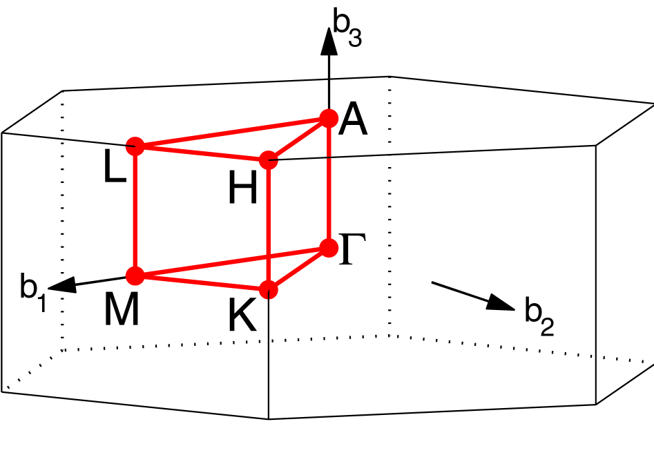 The easiest way to find the appropriate high symmetry path is by using
the AFLOW website. Go
to
http://aflow.org/aflow_online.html. This
website allows you to copy and paste a POSCAR file from VASP and will
automatically figure out the appropriate \(\mathbf{k}\)-space
path. Paste the POSCAR file to the input window and select ‘Kpath in
the reciprocal space for band structure calculations’, then hit the
Submit button on the top right of the window. This will generate a
file for use in electron band structure calculations. The
\(\mathbf{k}\)-path for the hexagonal lattice we are using is shown at
right.
The easiest way to find the appropriate high symmetry path is by using
the AFLOW website. Go
to
http://aflow.org/aflow_online.html. This
website allows you to copy and paste a POSCAR file from VASP and will
automatically figure out the appropriate \(\mathbf{k}\)-space
path. Paste the POSCAR file to the input window and select ‘Kpath in
the reciprocal space for band structure calculations’, then hit the
Submit button on the top right of the window. This will generate a
file for use in electron band structure calculations. The
\(\mathbf{k}\)-path for the hexagonal lattice we are using is shown at
right.
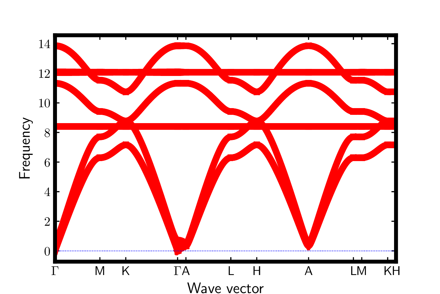
The output from AFLOW can now be used to generate band.conf. Our
path is
\(\Gamma\)-\(M\)-\(K\)-\(\Gamma\)-\(A\)-\(L\)-\(H\)-\(A\)-\(L\)-\(M\)-\(K\)-\(H\). The
band.conf file is:
ATOM_NAME = Mo S
DIM = 1 1 1
BAND =    0.000   0.000   0.000     0.500   0.000   0.000    0.3333  0.3333  0.000   0.000   0.000   0.000     0.000   0.000   0.500     0.500   0.000   0.500     0.3333  0.3333  0.500      0.000   0.000   0.500      0.500   0.000   0.500      0.500   0.000   0.000      0.3333  0.3333  0.000      0.3333  0.3333  0.500
BAND_LABELS= $\Gamma$ M K $\Gamma$ A L H A L M K H
Once you have created this file, run the following to get a plot of the band structure:
$ phonopy --readfc --dim="1 1 1" -p band.conf
The bands are shown below.
AFLOW citation: S. Curtarolo, W. Setyawan, G. L. W. Hart, M. Jahnatek, R. V. Chepulskii, R. H. Taylor, S. Wang, J. Xue, K. Yang, O. Levy, M. Mehl, H. T. Stokes, D. O. Demchenko, and D. Morgan, AFLOW: an automatic framework for high-throughput materials discovery, Comp. Mat. Sci. 58, 218-226 (2012). [doi=10.1016/j.commatsci.2012.02.005]
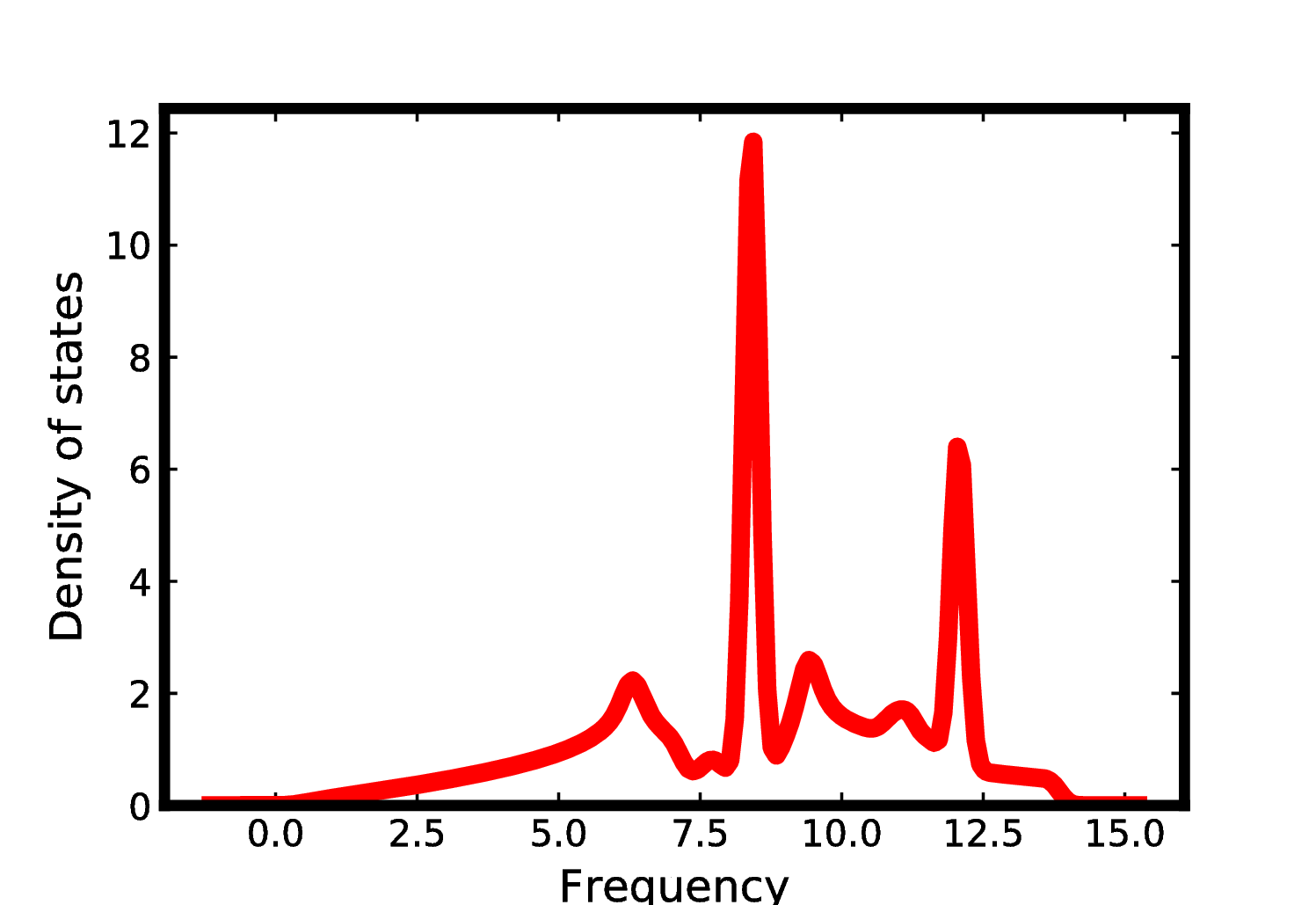
6. Phonon density of states
Once FORCE_CONSTANTS has been generated, it is easy to get the
phonon density of states:
$ phonopy --readfc --dim="1 1 1" --mesh="64 64 32" -p
This will produce the following plot:
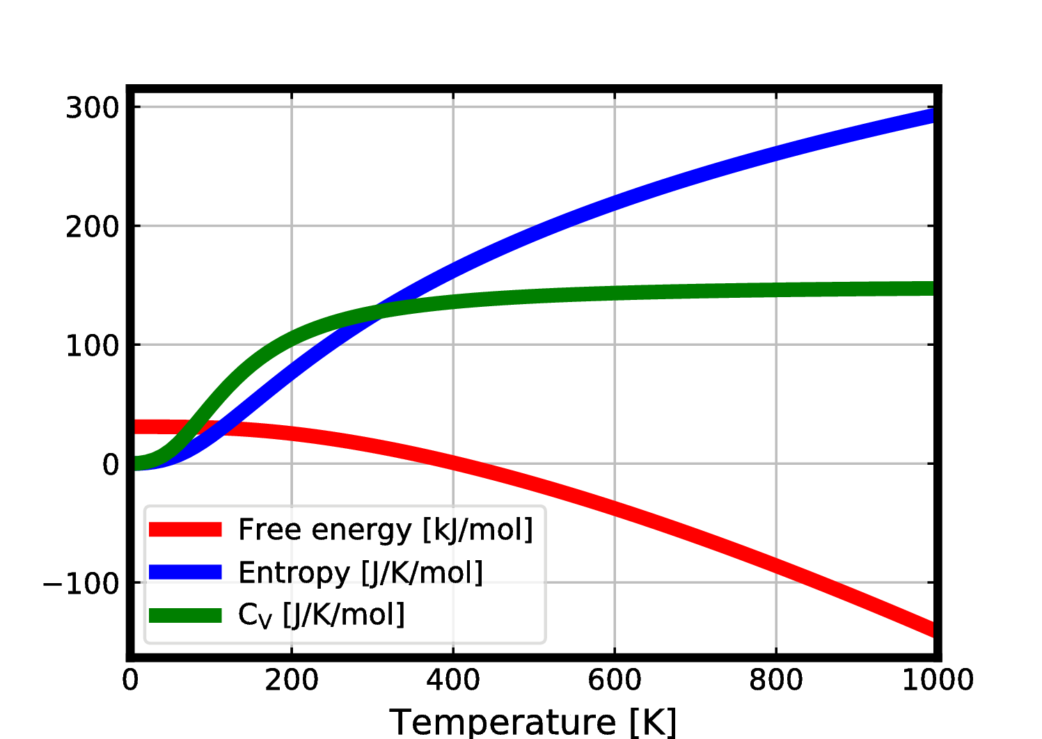
7. Free energy via Phonopy
To get a plot of values of thermal data and save values in “thermal.dat”, do the following:
$ phonopy --dim="1 1 1" --readfc -t -p --mesh="64 64 1" > thermal.dat
This will generate the following plot: