Band Structure via Quantum Espresso

Contents

• Prerequisites
• Overview
  • Files for this tutorial
  • General note about MPI
• 1. relax: Ionic relaxation
• 2. nscf: Performing a non-self-consistent field calculation
• 3. bands: Computing the band structure
  • a. Using xcrysden
  • b. Modifying the input file and running
• 4. plotbands: Plotting the bands

Prerequisites

Before getting started, you will want to make sure you have access to the following software:

1. Quantum Espresso 5.2.0 (or greater)
2. xcrysden 1.5.60 (other verisions likely work)

For installation instructions on these visit the software page.

Overview

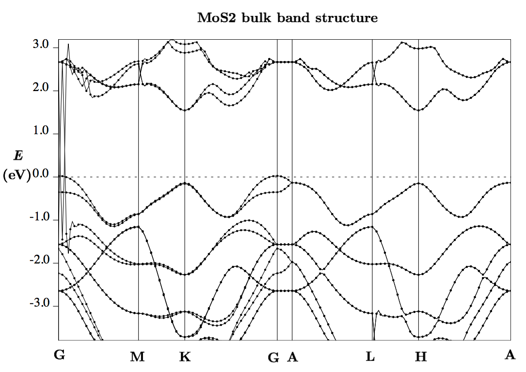
In this tutorial, we will calculate the band structure of bulk 2H-phase MoS$_2$. The bulk crystal is expected to be a semiconductor and have an indirect band gap. Indeed, we find both of these properties here using a PBE exchange-correlation potential. The results are very similar to the results in the VASP tutorial, which also used a PBE exchange-correlation potential.

Similar to VASP, a band structure calculation using Espresso involves a sequence of simulations. We can divide these into 4 parts:

1. Relaxation of the atomic positions (uses pw.x)
2. Non self-consistent (nscf) calculation (uses pw.x)
3. Band calculation (uses pw.x)
4. Plotting of the bands (uses bands.x and plotband.x)

Since there are 4 parts, I prefer setting up a directory structure that corresponds to each of the calculuations. In the root directory, I have

$ ls
1-relax/  2-nscf/  3-bands/  4-plotbands/  out/ 

Here, the numbered folders contain input files, while the out/ folder contains all of the Quantum Espresso-generated output, such as wavefunctions, xml files, and everything else that is generated when running Espresso. It is important to make sure that all input files in the numbered subdirectories have the same prefix and outdir, where outdir = '../out' inside each numbered folder. Below, we will go over the calculations done in each subfolder in detail.

Files for this tutorial

All files can be found at this git repo. Alternatively, clone them via

$ git clone https://github.com/rehnd/MoS2-band-structure.git

General note about MPI

For the first 3 calculations, you should run with the same number of processors for each of the calculations. The reason for this is that Espresso saves wave functions and other data in files corresponding to processor number. I have not experimented much with trying to change the number of processors for subsequent calcualtions; I always run with the same number of processors for steps 1-3, which all use pw.x.

However, step 4 (generating the bands files and plotting the bands) can be done in serial. This is because part 4 uses bands.x and plotband.x (not pw.x).

1. relax: Ionic relaxation

Input files for step 1: MoS2-2H.relax.pw.in

The first step is to relax the ion positions within the cell. This is done using pw.x.

After running pw.x (which is set up in the run.sbatch script), you will want to find the relaxed ion positions towards the end of the output file.

Steps for running the relaxation:

$ cd 1-relax
$ sbatch run.sbatch
$ cat *.out ## --> look for the ATOMIC_POSITIONS near the bottom of the output file

Above, the .sbatch file contains:

mpirun -np X /path/to/espresso/bin/pw.x < input-file.in > output-file.out

You should notice a folder called out in the parent directory of 1-relax.

2. nscf: Performing a non-self-consistent field calculation

Input files for step 2: MoS2-2H.nscf.pw.in

After running the relaxation, you will want to copy the final ion positions from the output of the relaxation and place them in an input file in 2-nscf. This file should look like the following: (link here)

There are 4 important differences between the input file from 1-relax and 2-nscf:

1. Under &control, you see calculation = 'nscf', instead of relax.
2. The ATOMIC_POSITIONS should be updated in the nscf calculation to be the ion positions after the relaxation.
3. The density of K_POINTS can (should) be higher in the nscf calculation
4. You can remove the &ions tag in the nscf calculation, because no ionic relaxation is needed. (If you forget to remove it, Espresso simply ignores the &ions tag by default)

3. bands: Computing the band structure

Input files for step 3: MoS2-2H.bands.pw.in

This step consists of 2 substeps. The first requirement is to choose a list of k-points for the band structure. The easiest way to do this is to use xcrysden, though you can use any method you like to do so. The second step is to modify the input file and run the calculation. Both steps will be discussed below.

a. Using xcrysden

First, you will want to install xcrysden. I have found that the easiest way on Mac is to use MacPorts. More information is found here.

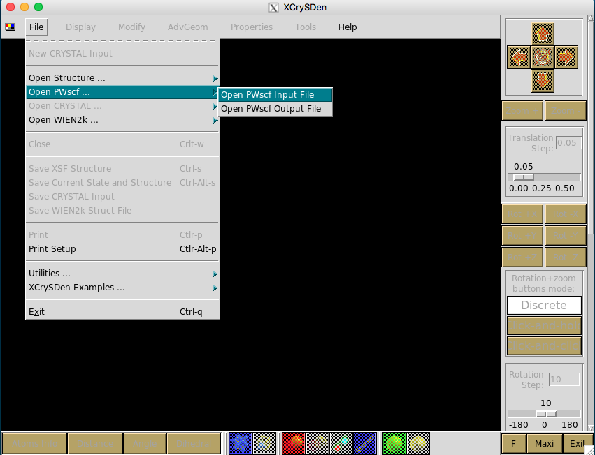
The next step is to open a PW input file:

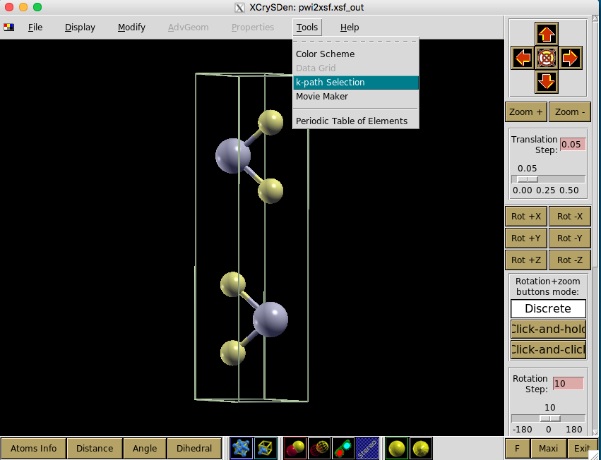
Once it is open, you should be able to rotate the unit cell around, as shown here:

To create a k-points list, go to the Tools tab:

Next, you need to select the k-space path that you want.

Useful: Check the “Display Reciprocal Vectors” box to see where the reciprocal space vectors are.

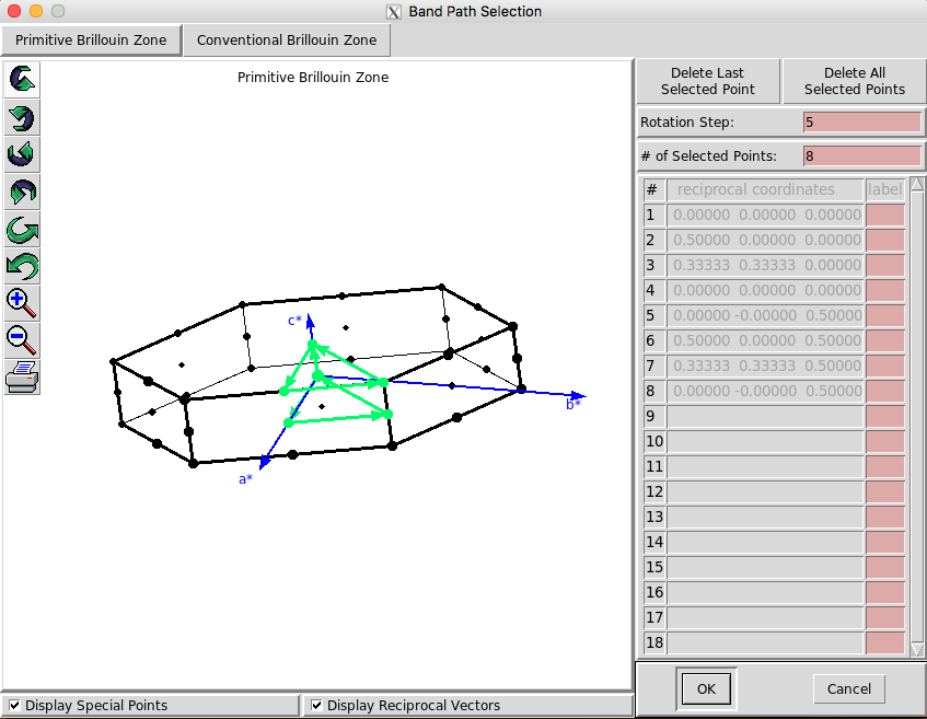
Next, seleck ‘Ok’ and choose the total number of k points along that path

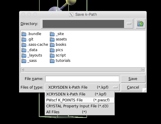
Finally, save as a .pwscf file. You need to enter a filename that ends with .pwscf to get it to work right.

This will output a file starting with K_POINTS, a line with the total number of k points in the file, and then a list of all k points. This file needs to be appended to the input file you will use to do the bands calculation, e.g.

$ cat output.pwscf >> inputfile.in

b. Modifying the input file and running

After generating a list of K_POINTS from xcrysden, you want to copy that list to the K_POINTS section of the input file. (You need to delete the previous K_POINTS list if you copied the input file from step 1 or 2.

There are 3 important things to keep in mind about this file:

1. The K_POINTS section of the file will be very different (and can be generated using xcrysden)
2. You should continue to use the relaxed ion positions in ATOMIC_POSITIONS
3. As with the nscf calculation, you do not need the &ions tag in the input file.

After adding the K_POINTS, run pw.x just like before on this new input file.

4. plotbands: Plotting the bands

This portion does not have to be done using MPI and should probably be run in serial. The input file for this is particularly simple, shown here:

&bands
  prefix   = "MoS2-2H"
  outdir   = "../out"
  filband  = "MoS2-2H.bands.dat"  ! Name of the output file with data
/

To run this, you can use the provided run.sbatch script in the 4-plotbands directory, or simply run the following from the commandline:

$ /path/to/espresso/bin/bands.x < input-file.in > output-file.out

After doing this, you will execute plotband.x, also located in bin. Executing this will prompt you for 1) an input file, 2) an energy range, 3) an output file(xmgr format) name, and 4) the output file name for the postscript (.ps) plot generated.

For this example, I use

$ /path/to/espresso/bin/plotband.x
Input file > MoS2-2H.bands.dat  # (same name specified by 'filband' above)
Reading xx bands at xxx k-points
Range:  -8.360  8.9960 Emin, Emax > -8.3, 9.0
...
output file (xmgr) > bands.xmgr
...
output file (ps) > bands.ps
Efermi > 3.0                    # you will have to choose this accordingly
deltaE, reference E > 1, 2      # deltaE = energy spacing on y-axis;
                                # reference E = zero of energy

After this, you should be able to open the .ps file and can rerun plotband.x as necessary to get the desired look.

After playing with parameters and adding axes labels, you should end up with something like this: